Ambit – A FEniCS-based cardiovascular multi-physics solver
- Author:
Dr.-Ing. Marc Hirschvogel
Preface
demos (with detailed setup descriptions) or amogst
the test cases in the folder tests.Installation
python3 -m pip install ambit-fe
or latest development version:
python3 -m pip install git+https://github.com/marchirschvogel/ambit.git
Alternatively, you can pull a pre-built Docker image with FEniCSx and Ambit installed:
docker pull ghcr.io/marchirschvogel/ambit:latest
If a Docker image for development is desired, the following image contains all dependencies needed to install and run Ambit:
docker pull ghcr.io/marchirschvogel/ambit:devenv
Ambit input
Here, a minimal Ambit input file is shown, exemplarily for a single-field problem. The mandatory parameter dictionaries to provide are input parameters (IO), global control parameters (CTR), time-integration parameters (TME), solver parameters (SOL), finite element parameters (FEM), and constitutive/material parameters (MAT). For multi-physics problems, each field needs individual time, finite element, and constitutive parameters.
#!/usr/bin/env python3

# Minimal input file for an elastodynamics problem

import ambit_fe
import numpy as np

def main():

    # Input/output
    IO = {"problem_type"        : "solid",                   # type of physics to solve
          "mesh_domain"         : "/path/mesh_d.xdmf",       # path to domain mesh
          "mesh_boundary"       : "/path/mesh_b.xdmf",       # ath to boundary mesh
          "meshfile_type"       : "HDF5",                    # encoding (HDF5 or ASCII)
          "write_results_every" : 1,                         # step frequency for output
          "output_path"         : "/path/...",               # path to output to
          "results_to_write"    : ["displacement",
                                   "vonmises_cauchystress"], # results to output
          "simname"             : "my_results_name"}         # midfix of output name

    # Global control
    CTR = {"maxtime"            : 1.0,  # maximum simulation time
           "dt"                 : 0.01} # time step size

    # Time discretization
    TME = {"timint"             : "genalpha", # time integration: Generalized-alpha
           "rho_inf_genalpha"   : 1.0}        # spectral radius of Gen-alpha scheme

    # Solver
    SOL = {"solve_type"         : "direct", # direct linear solver
           "tol_res"            : 1.0e-8,   # residual tolerance
           "tol_inc"            : 1.0e-8}   # increment tolerance

    # Finite element discretization
    FEM = {"order_disp"         : 1, # FEM degree for displacement field
           "quad_degree"        : 5} # quadrature scheme degree

    # Time curves
    class TC:
        # user defined load curves, to be used in boundary conditions (BC)
        def tc1(self, t):
            load_max = 5.0
            return load_max * np.sin(t)

    # Materials
    MAT = {"MAT1" : {"neohooke_dev" : {"mu" : 10.0},      # isochoric NeoHookean material
                     "ogden_vol"    : {"kappa" : 1.0e3},  # volumetric Ogden material
                     "inertia"      : {"rho0" : 1.0e-6}}} # density

    # Boundary conditions
    BC = {"dirichlet" : [{"id" : [<SURF_IDs>], # list of surfaces for Dirichlet BC
                          "dir" : "all",       # all directions
                          "val" : 0.0}],       # set to zero
          "neumann"   : [{"id" : [<SURF_IDs>], # list of surfaces for Neumann BC
                          "dir" : "xyz_ref",   # in cartesian reference directions
                          "curve" : [1,0,0]}]} # load in x-direction controlled by curve #1 (see time curves)

    # Problem setup
    problem = ambit_fe.ambit_main.Ambit(io_params=IO, ctrl_params=CTR, time_params=[TME], solver_params=SOL, fem_params=[FEM], constitutive_params=[MAT], boundary_conditions=[BC], time_curves=TC)

    # Run: solve the problem
    problem.solve_problem()

if __name__ == "__main__":

    main()
Physics Models
Solid mechanics
demos/solidproblem_type : "solid"Strong form
(1)\[\begin{split}\begin{aligned} \nabla_{0} \cdot \boldsymbol{P}(\boldsymbol{u},\boldsymbol{v}(\boldsymbol{u})) + \hat{\boldsymbol{b}}_{0} &= \rho_{0} \boldsymbol{a}(\boldsymbol{u}) &&\text{in} \; \mathit{\Omega}_{0} \times [0, T], \\ \boldsymbol{u} &= \hat{\boldsymbol{u}} &&\text{on} \; \mathit{\Gamma}_{0}^{\mathrm{D}} \times [0, T],\\ \boldsymbol{t}_{0} = \boldsymbol{P}\boldsymbol{n}_{0} &= \hat{\boldsymbol{t}}_{0} &&\text{on} \; \mathit{\Gamma}_{0}^{\mathrm{N}} \times [0, T],\\ \boldsymbol{u}(\boldsymbol{x}_{0},0) &= \hat{\boldsymbol{u}}_{0}(\boldsymbol{x}_{0}) &&\text{in} \; \mathit{\Omega}_{0},\\ \boldsymbol{v}(\boldsymbol{x}_{0},0) &= \hat{\boldsymbol{v}}_{0}(\boldsymbol{x}_{0}) &&\text{in} \; \mathit{\Omega}_{0}, \end{aligned}\end{split}\]
(2)\[\begin{split}\begin{aligned} \nabla_{0} \cdot \boldsymbol{P}(\boldsymbol{u},p,\boldsymbol{v}(\boldsymbol{u})) + \hat{\boldsymbol{b}}_{0} &= \rho_{0} \boldsymbol{a}(\boldsymbol{u}) &&\text{in} \; \mathit{\Omega}_{0} \times [0, T], \\ J(\boldsymbol{u})-1 &= 0 &&\text{in} \; \mathit{\Omega}_{0} \times [0, T], \\ \boldsymbol{u} &= \hat{\boldsymbol{u}} &&\text{on} \; \mathit{\Gamma}_{0}^{\mathrm{D}} \times [0, T],\\ \boldsymbol{t}_{0} = \boldsymbol{P}\boldsymbol{n}_{0} &= \hat{\boldsymbol{t}}_{0} &&\text{on} \; \mathit{\mathit{\Gamma}}_{0}^{\mathrm{N}} \times [0, T],\\ \boldsymbol{u}(\boldsymbol{x}_{0},0) &= \hat{\boldsymbol{u}}_{0}(\boldsymbol{x}_{0}) &&\text{in} \; \mathit{\mathit{\Omega}}_{0},\\ \boldsymbol{v}(\boldsymbol{x}_{0},0) &= \hat{\boldsymbol{v}}_{0}(\boldsymbol{x}_{0}) &&\text{in} \; \mathit{\mathit{\Omega}}_{0}, \end{aligned}\end{split}\]
Weak form
(3)\[\begin{aligned} r(\boldsymbol{u};\delta\boldsymbol{u}) := \delta \mathcal{W}_{\mathrm{kin}}(\boldsymbol{u};\delta\boldsymbol{u}) + \delta \mathcal{W}_{\mathrm{int}}(\boldsymbol{u};\delta\boldsymbol{u}) - \delta \mathcal{W}_{\mathrm{ext}}(\boldsymbol{u};\delta\boldsymbol{u}) = 0, \end{aligned}\]for all \(\delta\boldsymbol{u}\in\boldsymbol{\mathcal{V}}_{u}^{h}\)
(4)\[\begin{aligned} \delta \mathcal{W}_{\mathrm{kin}}(\boldsymbol{u};\delta\boldsymbol{u}) &= \int\limits_{\mathit{\Omega}_{0}} \rho_{0}\,\boldsymbol{a}(\boldsymbol{u}) \cdot \delta\boldsymbol{u} \,\mathrm{d}V \end{aligned}\]– Internal virtual work:
(5)\[\begin{aligned} \delta \mathcal{W}_{\mathrm{int}}(\boldsymbol{u};\delta\boldsymbol{u}) &= \int\limits_{\mathit{\Omega}_{0}} \boldsymbol{P}(\boldsymbol{u},\boldsymbol{v}(\boldsymbol{u})) : \nabla_{0} \delta\boldsymbol{u} \,\mathrm{d}V = \int\limits_{\mathit{\Omega}_{0}} \boldsymbol{S}(\boldsymbol{u},\boldsymbol{v}(\boldsymbol{u})) : \frac{1}{2}\delta\boldsymbol{C}(\boldsymbol{u}) \,\mathrm{d}V \end{aligned}\]– External virtual work:
conservative Neumann load:
(6)\[\begin{aligned} \delta \mathcal{W}_{\mathrm{ext}}(\delta\boldsymbol{u}) &= \int\limits_{\mathit{\Gamma}_{0}^{\mathrm{N}}} \hat{\boldsymbol{t}}_{0}(t) \cdot \delta\boldsymbol{u} \,\mathrm{d}A \end{aligned}\]Neumann pressure load in current normal direction:
(7)\[\begin{aligned} \delta \mathcal{W}_{\mathrm{ext}}(\boldsymbol{u};\delta\boldsymbol{u}) &= -\int\limits_{\mathit{\Gamma}_{0}^{\mathrm{N}}} \hat{p}(t)\,J \boldsymbol{F}^{-\mathrm{T}}\boldsymbol{n}_{0} \cdot \delta\boldsymbol{u} \,\mathrm{d}A \end{aligned}\]general Neumann load in current direction:
(8)\[\begin{aligned} \delta \mathcal{W}_{\mathrm{ext}}(\boldsymbol{u};\delta\boldsymbol{u}) &= \int\limits_{\mathit{\Gamma}_0} J\boldsymbol{F}^{-\mathrm{T}}\,\hat{\boldsymbol{t}}_{0}(t) \cdot \delta\boldsymbol{u} \,\mathrm{d}A \end{aligned}\]body force:
(9)\[\begin{aligned} \delta \mathcal{W}_{\mathrm{ext}}(\delta\boldsymbol{u}) &= \int\limits_{\mathit{\Omega}_{0}} \hat{\boldsymbol{b}}_{0}(t) \cdot \delta\boldsymbol{u} \,\mathrm{d}V \end{aligned}\]generalized Robin condition:
(10)\[\begin{aligned} \delta \mathcal{W}_{\mathrm{ext}}(\boldsymbol{u};\delta\boldsymbol{u}) &= -\int\limits_{\mathit{\Gamma}_{0}^{\mathrm{R}}} \left[k\,\boldsymbol{u} + c\,\boldsymbol{v}(\boldsymbol{u})\right] \cdot \delta\boldsymbol{u}\,\mathrm{d}A \end{aligned}\]generalized Robin condition in reference surface normal direction:
(11)\[\begin{aligned} \delta \mathcal{W}_{\mathrm{ext}}(\boldsymbol{u};\delta\boldsymbol{u}) &= -\int\limits_{\mathit{\Gamma}_{0}^{\mathrm{R}}} (\boldsymbol{n}_0 \otimes \boldsymbol{n}_0)\left[k\,\boldsymbol{u} + c\,\boldsymbol{v}(\boldsymbol{u})\right] \cdot \delta\boldsymbol{u}\,\mathrm{d}A \end{aligned}\]
(12)\[\begin{split}\begin{aligned} r_u(\boldsymbol{u},p;\delta\boldsymbol{u}) &:= \delta \mathcal{W}_{\mathrm{kin}}(\boldsymbol{u};\delta\boldsymbol{u}) + \delta \mathcal{W}_{\mathrm{int}}(\boldsymbol{u},p;\delta\boldsymbol{u}) - \delta \mathcal{W}_{\mathrm{ext}}(\boldsymbol{u};\delta\boldsymbol{u}) = 0, \\ r_p(\boldsymbol{u};\delta p) &:= \delta \mathcal{W}_{\mathrm{pres}}(\boldsymbol{u};\delta p) = 0, \end{aligned}\end{split}\]for all \((\delta\boldsymbol{u},\delta p) \in \boldsymbol{\mathcal{V}}_{u}^{h} \times \mathcal{V}_{p}^{h}\)
(13)\[\begin{aligned} \delta \mathcal{W}_{\mathrm{int}}(\boldsymbol{u},p;\delta\boldsymbol{u}) &= \int\limits_{\mathit{\Omega}_{0}} \boldsymbol{P}(\boldsymbol{u},p,\boldsymbol{v}(\boldsymbol{u})) : \nabla_{0} \delta\boldsymbol{u} \,\mathrm{d}V = \int\limits_{\mathit{\Omega}_{0}} \boldsymbol{S}(\boldsymbol{u},p,\boldsymbol{v}(\boldsymbol{u})) : \frac{1}{2}\delta\boldsymbol{C}(\boldsymbol{u}) \,\mathrm{d}V \end{aligned}\]– Pressure virtual work:
(14)\[\begin{aligned} \delta \mathcal{W}_{\mathrm{pres}}(\boldsymbol{u};\delta p) &= \int\limits_{\mathit{\Omega}_{0}} (J(\boldsymbol{u}) - 1) \,\delta p \,\mathrm{d}V \end{aligned}\]
\[\begin{aligned} \boldsymbol{S} = 2\frac{\partial\mathit{\Psi}}{\partial \boldsymbol{C}} \end{aligned}\]
"neohooke_dev"\[\begin{aligned} \mathit{\Psi} &= \frac{\mu}{2}\left(\bar{I}_C - 3\right) \end{aligned}\]
"holzapfelogden_dev"\[\begin{split}\begin{aligned} \mathit{\Psi} &= \frac{a_0}{2b_0}\left(e^{b_0(\bar{I}_C - 3)} - 1\right) + \sum\limits_{i\in\{f,s\}}\frac{a_i}{2b_i}\left(e^{b_i(I_{4,i}-1)^2}-1\right) + \frac{a_{fs}}{2b_{fs}}\left(e^{b_{fs}I_{8}^2} - 1\right), \\ & I_{4,f} = \boldsymbol{f}_0 \cdot \boldsymbol{C}\boldsymbol{f}_0, \quad I_{4,s} = \boldsymbol{s}_0 \cdot \boldsymbol{C}\boldsymbol{s}_0, \quad I_8 = \boldsymbol{f}_0 \cdot \boldsymbol{C}\boldsymbol{s}_0 \end{aligned}\end{split}\]
– viscous material models
timint : "static"\[\begin{aligned} \delta \mathcal{W}_{\mathrm{int}}(\boldsymbol{u}_{n+1};\delta\boldsymbol{u}) - \delta \mathcal{W}_{\mathrm{ext}}(\boldsymbol{u}_{n+1};\delta\boldsymbol{u}) = 0, \quad \forall \; \delta\boldsymbol{u}\end{aligned}\]– Generalized-alpha time scheme
timint : "genalpha"\[\begin{split}\begin{aligned} \boldsymbol{v}_{n+1} &= \frac{\gamma}{\beta\Delta t}(\boldsymbol{u}_{n+1}-\boldsymbol{u}_{n}) - \frac{\gamma-\beta}{\beta} \boldsymbol{v}_{n} - \frac{\gamma-2\beta}{2\beta}\Delta t\,\boldsymbol{a}_{n} \\ \boldsymbol{a}_{n+1} &= \frac{1}{\beta\Delta t^2}(\boldsymbol{u}_{n+1}-\boldsymbol{u}_{n}) - \frac{1}{\beta\Delta t} \boldsymbol{v}_{n} - \frac{1-2\beta}{2\beta}\boldsymbol{a}_{n} \end{aligned}\end{split}\]
option
eval_nonlin_terms : "midpoint":(15)\[\begin{split}\begin{aligned} \boldsymbol{u}_{n+1-\alpha_{\mathrm{f}}} &= (1-\alpha_{\mathrm{f}})\boldsymbol{u}_{n+1} + \alpha_{\mathrm{f}} \boldsymbol{v}_{n} \\ \boldsymbol{v}_{n+1-\alpha_{\mathrm{f}}} &= (1-\alpha_{\mathrm{f}})\boldsymbol{v}_{n+1} + \alpha_{\mathrm{f}} \boldsymbol{v}_{n} \\ \boldsymbol{a}_{n+1-\alpha_{\mathrm{m}}} &= (1-\alpha_{\mathrm{m}})\boldsymbol{a}_{n+1} + \alpha_{\mathrm{m}} \boldsymbol{a}_{n} \end{aligned}\end{split}\]\[\begin{aligned} \delta \mathcal{W}_{\mathrm{kin}}(\boldsymbol{a}_{n+1-\alpha_{m}};\delta\boldsymbol{u}) + \delta \mathcal{W}_{\mathrm{int}}(\boldsymbol{u}_{n+1-\alpha_{f}};\delta\boldsymbol{u}) - \delta \mathcal{W}_{\mathrm{ext}}(\boldsymbol{u}_{n+1-\alpha_{f}};\delta\boldsymbol{u}) = 0, \quad \forall \; \delta\boldsymbol{u}\end{aligned}\]
option
eval_nonlin_terms : "trapezoidal":\[\begin{split}\begin{aligned} &(1-\alpha_{\mathrm{m}})\,\delta \mathcal{W}_{\mathrm{kin}}(\boldsymbol{a}_{n+1};\delta\boldsymbol{u}) + \alpha_{\mathrm{m}}\,\delta \mathcal{W}_{\mathrm{kin}}(\boldsymbol{a}_{n};\delta\boldsymbol{u}) + \\ & (1-\alpha_{\mathrm{f}})\,\delta \mathcal{W}_{\mathrm{int}}(\boldsymbol{u}_{n+1};\delta\boldsymbol{u}) + \alpha_{\mathrm{f}}\,\delta \mathcal{W}_{\mathrm{int}}(\boldsymbol{u}_{n};\delta\boldsymbol{u}) - \\ & (1-\alpha_{f})\,\delta \mathcal{W}_{\mathrm{ext}}(\boldsymbol{u}_{n+1};\delta\boldsymbol{u}) - \alpha_{\mathrm{f}}\,\delta \mathcal{W}_{\mathrm{ext}}(\boldsymbol{u}_{n};\delta\boldsymbol{u}) = 0, \quad \forall \; \delta\boldsymbol{u}\end{aligned}\end{split}\]
– One-Step-theta time scheme timint : "ost"
option
eval_nonlin_terms : "midpoint":
option
eval_nonlin_terms : "trapezoidal":
"midpoint" and "trapezoidal" for all
linear terms, e.g. \(\delta \mathcal{W}_{\mathrm{kin}}\), or for
no or only linear dependence of
\(\delta \mathcal{W}_{\mathrm{ext}}\) on the solution.\[\begin{aligned} \delta \mathcal{W}_{\mathrm{pres}}(\boldsymbol{u}_{n+1};\delta p) = 0, \quad \forall \; \delta p, \end{aligned}\]and the pressure in \(\delta \mathcal{W}_{\mathrm{int}}\) is set according to ([equation-solid-midpoint-genalpha]) or ([equation-solid-midpoint-ost]), respectively.
(17)\[\begin{aligned} \left.\boldsymbol{\mathsf{r}}_{u}(\boldsymbol{\mathsf{u}})\right|_{n+1} = \boldsymbol{\mathsf{0}} \end{aligned}\]
– Discrete linear system to solve in each Newton iteration \(k\) (displacement-based):
– Discrete nonlinear system to solve in each time step \(n\) (incompressible):
– Discrete linear system to solve in each Newton iteration \(k\) (incompressible):
Fluid mechanics
Eulerian reference frame
demos/fluidfluid(21)\[\begin{split}\begin{aligned} \rho\left(\frac{\partial\boldsymbol{v}}{\partial t} + (\nabla\boldsymbol{v})\,\boldsymbol{v}\right) &= \nabla \cdot \boldsymbol{\sigma}(\boldsymbol{v},p) + \hat{\boldsymbol{b}} &&\text{in} \; \mathit{\mathit{\Omega}}_t \times [0, T], \\ \nabla\cdot \boldsymbol{v} &= 0 &&\text{in} \; \mathit{\mathit{\Omega}}_t \times [0, T],\\ \boldsymbol{v} &= \hat{\boldsymbol{v}} &&\text{on} \; \mathit{\mathit{\Gamma}}_t^{\mathrm{D}} \times [0, T],\\ \boldsymbol{t} = \boldsymbol{\sigma}\boldsymbol{n} &= \hat{\boldsymbol{t}} &&\text{on} \; \mathit{\mathit{\Gamma}}_t^{\mathrm{N}} \times [0, T],\\ \boldsymbol{v}(\boldsymbol{x},0) &= \hat{\boldsymbol{v}}_{0}(\boldsymbol{x}) &&\text{in} \; \mathit{\mathit{\Omega}}_t, \end{aligned}\end{split}\]
with a Newtonian fluid constitutive law
where \(\eta\) is the dynamic viscosity
(22)\[\begin{split}\begin{aligned} r_v(\boldsymbol{v},p;\delta\boldsymbol{v}) &:= \delta \mathcal{P}_{\mathrm{kin}}(\boldsymbol{v};\delta\boldsymbol{v}) + \delta \mathcal{P}_{\mathrm{int}}(\boldsymbol{v},p;\delta\boldsymbol{v}) - \delta \mathcal{P}_{\mathrm{ext}}(\boldsymbol{v};\delta\boldsymbol{v}) = 0, \quad \\ r_p(\boldsymbol{v};\delta p) &:= \delta \mathcal{P}_{\mathrm{pres}}(\boldsymbol{v};\delta p) = 0, \end{aligned}\end{split}\]for all \((\delta\boldsymbol{v},\delta p) \in \boldsymbol{\mathcal{V}}_{v}^{h} \times \mathcal{V}_{p}^{h}\)
– Kinetic virtual power:
– Internal virtual power:
– Pressure virtual power:
conservative Neumann load:
(26)\[\begin{aligned} \delta \mathcal{P}_{\mathrm{ext}}(\delta\boldsymbol{v}) &= \int\limits_{\mathit{\Gamma}_t^{\mathrm{N}}} \hat{\boldsymbol{t}}(t) \cdot \delta\boldsymbol{v} \,\mathrm{d}a \end{aligned}\]pressure Neumann load:
(27)\[\begin{aligned} \delta \mathcal{P}_{\mathrm{ext}}(\delta\boldsymbol{v}) &= -\int\limits_{\mathit{\Gamma}_t^{\mathrm{N}}} \hat{p}(t)\,\boldsymbol{n} \cdot \delta\boldsymbol{v} \,\mathrm{d}a \end{aligned}\]body force:
(28)\[\begin{aligned} \delta \mathcal{P}_{\mathrm{ext}}(\delta\boldsymbol{v}) &= \int\limits_{\mathit{\Omega}_t} \hat{\boldsymbol{b}}(t) \cdot \delta\boldsymbol{v} \,\mathrm{d}V \end{aligned}\]
"stabilization" : {"scheme" : <SCHEME>, "vscale" : 1e3, "dscales" : [<d1>,<d2>,<d3>],
                   "symmetric" : False, "reduced_scheme" : False}
"supg_pspg":\[\begin{split}\begin{aligned} r_v \leftarrow r_v &+ \frac{1}{\rho}\int\limits_{\mathit{\Omega}_t} \tau_{\mathrm{SUPG}}\,(\nabla\delta\boldsymbol{v})\,\boldsymbol{v} \cdot \left(\rho\left(\frac{\partial \boldsymbol{v}}{\partial t} + (\nabla\boldsymbol{v})\,\boldsymbol{v}\right) - \nabla \cdot \boldsymbol{\sigma}(\boldsymbol{v},p)\right)\,\mathrm{d}v \\ & + \int\limits_{\mathit{\Omega}_t} \tau_{\mathrm{LSIC}}\,\rho\,(\nabla\cdot\delta\boldsymbol{v})(\nabla\cdot\boldsymbol{v})\,\mathrm{d}v \end{aligned}\end{split}\]– Pressure residual operator in ([equation-fluid-weak-form]) is augmented by the following terms:
\[\begin{aligned} r_p \leftarrow r_p &+ \frac{1}{\rho}\int\limits_{\mathit{\Omega}_t} \tau_{\mathrm{PSPG}}\,(\nabla\delta p) \cdot \left(\rho\left(\frac{\partial \boldsymbol{v}}{\partial t} + (\nabla\boldsymbol{v})\,\boldsymbol{v}\right) - \nabla \cdot \boldsymbol{\sigma}(\boldsymbol{v},p)\right)\,\mathrm{d}v \end{aligned}\]
– Discrete nonlinear system to solve in each time step \(n\):
– Discrete linear system to solve in each Newton iteration \(k\):
– Note that \(\boldsymbol{\mathsf{K}}_{pp}\) is zero for Taylor-Hood elements (without stabilization)
ALE reference frame
fluid_ale(31)\[\begin{split}\begin{aligned} \nabla_{0} \cdot \boldsymbol{\sigma}^{\mathrm{G}}(\boldsymbol{d}) &= \boldsymbol{0} &&\text{in} \; \mathit{\mathit{\Omega}}_0, \\ \boldsymbol{d} &= \hat{\boldsymbol{d}} &&\text{on} \; \mathit{\mathit{\Gamma}}_0^{\mathrm{D}}, \end{aligned}\end{split}\]– ALE material
linelast:\[\begin{aligned} \boldsymbol{\sigma}^{\mathrm{G}}(\boldsymbol{d}) = 2\mu \,\boldsymbol{\varepsilon} + \lambda \,\mathrm{tr}\boldsymbol{\varepsilon}\,\boldsymbol{I}, \qquad \text{with}\quad \boldsymbol{\varepsilon} = \frac{1}{2}\left(\nabla_0\boldsymbol{d} + (\nabla_0\boldsymbol{d})^{\mathrm{T}}\right) \end{aligned}\]– ALE material
diffusion:\[\begin{aligned} \boldsymbol{\sigma}^{\mathrm{G}}(\boldsymbol{d}) = D \,\nabla_0\boldsymbol{d} \end{aligned}\]– ALE material
neohooke(fully nonlinear model):\[\begin{aligned} \boldsymbol{\sigma}^{\mathrm{G}}(\boldsymbol{d}) = \frac{\partial \mathit{\Psi}}{\partial \widehat{\boldsymbol{F}}}, \qquad \text{with}\quad \mathit{\Psi} = \frac{\mu}{2}\left(\mathrm{tr}(\widehat{\boldsymbol{F}}^{\mathrm{T}}\widehat{\boldsymbol{F}}) - 3\right) + \frac{\mu}{2\beta} \left(\widehat{J}^{-2\beta} - 1\right) \end{aligned}\]
– weak form:
(33)\[\begin{split}\begin{aligned} \widehat{J}\rho\left(\left.\frac{\partial\boldsymbol{v}}{\partial t}\right|_{\boldsymbol{x}_{0}} + (\nabla_0\boldsymbol{v}\,\widehat{\boldsymbol{F}}^{-1})\,(\boldsymbol{v}-\widehat{\boldsymbol{w}})\right) &= \nabla_{0} \cdot\left(\widehat{J}\boldsymbol{\sigma} \widehat{\boldsymbol{F}}^{-\mathrm{T}}\right) + \widehat{J}\hat{\boldsymbol{b}} &&\text{in} \; \mathit{\mathit{\Omega}}_0 \times [0, T],\\ \nabla_{0}\cdot\left(\widehat{J}\widehat{\boldsymbol{F}}^{-1}\boldsymbol{v}\right) &= 0 &&\text{in} \; \mathit{\mathit{\Omega}}_0 \times [0, T],\\ \boldsymbol{v} &= \hat{\boldsymbol{v}} &&\text{on} \; \mathit{\mathit{\Gamma}}_0^{\mathrm{D}} \times [0, T], \\ \boldsymbol{t} = \boldsymbol{\sigma}\boldsymbol{n} &= \hat{\boldsymbol{t}} &&\text{on} \; \mathit{\mathit{\Gamma}}_0^{\mathrm{N}} \times [0, T], \\ \boldsymbol{v}(\boldsymbol{x},0) &= \hat{\boldsymbol{v}}_{0}(\boldsymbol{x}) &&\text{in} \; \mathit{\mathit{\Omega}}_0, \end{aligned}\end{split}\]
with a Newtonian fluid constitutive law
(34)\[\begin{split}\begin{aligned} r_v(\boldsymbol{v},p,\boldsymbol{d};\delta\boldsymbol{v}) &:= \delta \mathcal{P}_{\mathrm{kin}}(\boldsymbol{v},\boldsymbol{d};\delta\boldsymbol{v}) + \delta \mathcal{P}_{\mathrm{int}}(\boldsymbol{v},p,\boldsymbol{d};\delta\boldsymbol{v}) - \delta \mathcal{P}_{\mathrm{ext}}(\boldsymbol{v},\boldsymbol{d};\delta\boldsymbol{v}) = 0, \\ r_p(\boldsymbol{v},\boldsymbol{d};\delta p) &:= \delta \mathcal{P}_{\mathrm{pres}}(\boldsymbol{v},\boldsymbol{d};\delta p) = 0, \\ r_{d}(\boldsymbol{d};\delta\boldsymbol{d}) &= 0, \end{aligned}\end{split}\]for all \((\delta\boldsymbol{v},\delta p,\delta\boldsymbol{d}) \in \boldsymbol{\mathcal{V}}_{v}^{h} \times \mathcal{V}_{p}^{h} \times \boldsymbol{\mathcal{V}}_{d}^{h}\)
– Kinetic virtual power:
– Internal virtual power:
– Pressure virtual power:
conservative Neumann load:
\[\begin{aligned} \delta \mathcal{P}_{\mathrm{ext}}(\delta\boldsymbol{v}) &= \int\limits_{\mathit{\Gamma}_0^{\mathrm{N}}} \hat{\boldsymbol{t}}(t) \cdot \delta\boldsymbol{v} \,\mathrm{d}A \end{aligned}\]pressure Neumann load:
\[\begin{aligned} \delta \mathcal{P}_{\mathrm{ext}}(\boldsymbol{d};\delta\boldsymbol{v}) &= -\int\limits_{\mathit{\Gamma}_0^{\mathrm{N}}} \hat{p}(t)\,\widehat{J}\widehat{\boldsymbol{F}}^{-\mathrm{T}}\boldsymbol{n}_{0} \cdot \delta\boldsymbol{v} \,\mathrm{d}A \end{aligned}\]body force:
\[\begin{aligned} \delta \mathcal{P}_{\mathrm{ext}}(\boldsymbol{d};\delta\boldsymbol{v}) &= \int\limits_{\mathit{\Omega}_0} \widehat{J}\,\hat{\boldsymbol{b}}(t) \cdot \delta\boldsymbol{v} \,\mathrm{d}V \end{aligned}\]
"supg_pspg":\[\begin{split}\begin{aligned} r_v \leftarrow r_v &+ \frac{1}{\rho}\int\limits_{\mathit{\Omega}_0}\widehat{J}\, \tau_{\mathrm{SUPG}}\,(\nabla_0\delta\boldsymbol{v}\,\widehat{\boldsymbol{F}}^{-1})\,\boldsymbol{v}\;\cdot \\ & \qquad\quad \cdot\left(\widehat{J}\rho\left(\left.\frac{\partial \boldsymbol{v}}{\partial t}\right|_{\boldsymbol{x}_{0}} + (\nabla_0\boldsymbol{v}\,\widehat{\boldsymbol{F}}^{-1})\,(\boldsymbol{v}-\widehat{\boldsymbol{w}})\right) - \nabla_{0}\cdot\left(\widehat{J}\boldsymbol{\sigma}\widehat{\boldsymbol{F}}^{-\mathrm{T}}\right)\right)\,\mathrm{d}V \\ & + \int\limits_{\mathit{\Omega}_0}\widehat{J}\, \tau_{\mathrm{LSIC}}\,\rho\,(\nabla_{0}\delta\boldsymbol{v} : \widehat{\boldsymbol{F}}^{-\mathrm{T}})(\nabla_{0}\boldsymbol{v} : \widehat{\boldsymbol{F}}^{-\mathrm{T}})\,\mathrm{d}V \end{aligned}\end{split}\]– Pressure residual operator in ([equation-fluid-ale-weak-form]) is augmented by the following terms:
\[\begin{split}\begin{aligned} r_p \leftarrow r_p &+ \frac{1}{\rho}\int\limits_{\mathit{\Omega}_0}\widehat{J}\, \tau_{\mathrm{PSPG}}\,(\widehat{\boldsymbol{F}}^{-\mathrm{T}}\nabla_{0}\delta p) \;\cdot \\ & \qquad\quad \cdot \left(\widehat{J}\rho\left(\left.\frac{\partial \boldsymbol{v}}{\partial t}\right|_{\boldsymbol{x}_{0}} + (\nabla_0\boldsymbol{v}\,\widehat{\boldsymbol{F}}^{-1})\,(\boldsymbol{v}-\widehat{\boldsymbol{w}})\right) - \nabla_{0}\cdot\left(\widehat{J}\boldsymbol{\sigma}\widehat{\boldsymbol{F}}^{-\mathrm{T}}\right)\right)\,\mathrm{d}V \end{aligned}\end{split}\]
– Discrete nonlinear system to solve in each time step \(n\):
– Discrete linear system to solve in each Newton iteration \(k\):
– note that \(\boldsymbol{\mathsf{K}}_{pp}\) is zero for Taylor-Hood elements (without stabilization)
0D flow: Lumped parameter models
demos/flow0dflow0d2-element Windkessel
2elwindkessel4-element Windkessel (inertance parallel to impedance)
4elwindkesselLpZ4-element Windkessel (inertance serial to impedance)
4elwindkesselLsZIn-outflow CRL link
CRLinoutlinkSystemic and pulmonary circulation
syspulwith:
and:
The volume \(V\) of the heart chambers (0D) is modeled by the volume-pressure relationship
with the unstressed volume \(V_{\mathrm{u}}\) and the time-varying elastance
where \(E_{\mathrm{max}}\) and \(E_{\mathrm{min}}\) denote the maximum and minimum elastance, respectively. The normalized activation function \(\hat{y}(t)\) is input by the user.
Flow-pressure relations for the four valves, eq. ([eq:mv_flow]), ([eq:av_flow]), ([eq:tv_flow]), ([eq:pv_flow]), are functions of the pressure difference \(p-p_{\mathrm{open}}\) across the valve. The following valve models can be defined:
Valve model pwlin_pres:
Remark: Non-smooth flow-pressure relationship
Valve model pwlin_time:
Remark: Non-smooth flow-pressure relationship with resistance only dependent on timings, not the pressure difference!
Valve model smooth_pres_resistance:
Remark: Smooth but potentially non-convex flow-pressure relationship!
Valve model smooth_pres_momentum:
with
and
with
pwlin_pres for \(\epsilon=0\)pw_pres_regurg:\[\begin{split}\begin{aligned} q(p-p_{\mathrm{open}}) = \begin{cases} c A_{\mathrm{o}} \sqrt{p-p_{\mathrm{open}}}, & p < p_{\mathrm{open}} \\ \frac{p-p_{\mathrm{open}}}{R_{\min}}, & p \geq p_{\mathrm{open}} \end{cases} \end{aligned}\end{split}\]Remark: Model to allow a regurgitant valve in the closed state, degree of regurgitation can be varied by specifying the valve regurgitant area \(A_{\mathrm{o}}\)
ZCRp_CRd_lr\[\begin{split}\begin{aligned} &C_{\mathrm{cor,p}}^{\mathrm{sys},\ell} \left(\frac{\mathrm{d}p_{\mathrm{ar}}^{\mathrm{sys},\ell}}{\mathrm{d}t}-Z_{\mathrm{cor,p}}^{\mathrm{sys},\ell}\frac{\mathrm{d}q_{\mathrm{cor,p,in}}^{\mathrm{sys},\ell}}{\mathrm{d}t}\right) = q_{\mathrm{cor,p,in}}^{\mathrm{sys},\ell} - q_{\mathrm{cor,p}}^{\mathrm{sys},\ell} && \text{left coronary proximal flow balance}\\ &R_{\mathrm{cor,p}}^{\mathrm{sys},\ell}\,q_{\mathrm{cor,p}}^{\mathrm{sys},\ell}=p_{\mathrm{ar}}^{\mathrm{sys}}-p_{\mathrm{cor,d}}^{\mathrm{sys},\ell} - Z_{\mathrm{cor,p}}^{\mathrm{sys},\ell}\,q_{\mathrm{cor,p,in}}^{\mathrm{sys},\ell} && \text{left coronary proximal momentum}\\ &C_{\mathrm{cor,d}}^{\mathrm{sys},\ell} \frac{\mathrm{d}(p_{\mathrm{cor,d}}^{\mathrm{sys},\ell}-p_{\mathrm{v}}^{\ell})}{\mathrm{d}t} = q_{\mathrm{cor,p}}^{\mathrm{sys},\ell} - q_{\mathrm{cor,d}}^{\mathrm{sys},\ell} && \text{left coronary distal flow balance}\\ &R_{\mathrm{cor,d}}^{\mathrm{sys},\ell}\,q_{\mathrm{cor,d}}^{\mathrm{sys},\ell}=p_{\mathrm{cor,d}}^{\mathrm{sys},\ell}-p_{\mathrm{at}}^{r} && \text{left coronary distal momentum}\\ &C_{\mathrm{cor,p}}^{\mathrm{sys},r} \left(\frac{\mathrm{d}p_{\mathrm{ar}}^{\mathrm{sys},r}}{\mathrm{d}t}-Z_{\mathrm{cor,p}}^{\mathrm{sys},r}\frac{\mathrm{d}q_{\mathrm{cor,p,in}}^{\mathrm{sys},r}}{\mathrm{d}t}\right) = q_{\mathrm{cor,p,in}}^{\mathrm{sys},r} - q_{\mathrm{cor,p}}^{\mathrm{sys},r} && \text{right coronary proximal flow balance}\\ &R_{\mathrm{cor,p}}^{\mathrm{sys},r}\,q_{\mathrm{cor,p}}^{\mathrm{sys},r}=p_{\mathrm{ar}}^{\mathrm{sys}}-p_{\mathrm{cor,d}}^{\mathrm{sys},r} - Z_{\mathrm{cor,p}}^{\mathrm{sys},r}\,q_{\mathrm{cor,p,in}}^{\mathrm{sys},r} && \text{right coronary proximal momentum}\\ &C_{\mathrm{cor,d}}^{\mathrm{sys},r} \frac{\mathrm{d}(p_{\mathrm{cor,d}}^{\mathrm{sys},r}-p_{\mathrm{v}}^{\ell})}{\mathrm{d}t} = q_{\mathrm{cor,p}}^{\mathrm{sys},r} - q_{\mathrm{cor,d}}^{\mathrm{sys},r} && \text{right coronary distal flow balance}\nonumber\\ &R_{\mathrm{cor,d}}^{\mathrm{sys},r}\,q_{\mathrm{cor,d}}^{\mathrm{sys},r}=p_{\mathrm{cor,d}}^{\mathrm{sys},r}-p_{\mathrm{at}}^{r} && \text{right coronary distal momentum}\\ &0=q_{\mathrm{cor,d}}^{\mathrm{sys},\ell}+q_{\mathrm{cor,d}}^{\mathrm{sys},r}-q_{\mathrm{cor,d,out}}^{\mathrm{sys}} && \text{distal coronary junction flow balance} \end{aligned}\end{split}\]
ZCRp_CRd\[\begin{split}\begin{aligned} &C_{\mathrm{cor,p}}^{\mathrm{sys}} \left(\frac{\mathrm{d}p_{\mathrm{ar}}^{\mathrm{sys}}}{\mathrm{d}t}-Z_{\mathrm{cor,p}}^{\mathrm{sys}}\frac{\mathrm{d}q_{\mathrm{cor,p,in}}^{\mathrm{sys}}}{\mathrm{d}t}\right) = q_{\mathrm{cor,p,in}}^{\mathrm{sys}} - q_{\mathrm{cor,p}}^{\mathrm{sys}} && \text{coronary proximal flow balance}\\ &R_{\mathrm{cor,p}}^{\mathrm{sys}}\,q_{\mathrm{cor,p}}^{\mathrm{sys}}=p_{\mathrm{ar}}^{\mathrm{sys}}-p_{\mathrm{cor,d}}^{\mathrm{sys}} - Z_{\mathrm{cor,p}}^{\mathrm{sys}}\,q_{\mathrm{cor,p,in}}^{\mathrm{sys}} && \text{coronary proximal momentum}\nonumber\\ &C_{\mathrm{cor,d}}^{\mathrm{sys}} \frac{\mathrm{d}(p_{\mathrm{cor,d}}^{\mathrm{sys}}-p_{\mathrm{v}}^{\ell})}{\mathrm{d}t} = q_{\mathrm{cor,p}}^{\mathrm{sys}} - q_{\mathrm{cor,d}}^{\mathrm{sys}} && \text{coronary distal flow balance}\\ &R_{\mathrm{cor,d}}^{\mathrm{sys}}\,q_{\mathrm{cor,d}}^{\mathrm{sys}}=p_{\mathrm{cor,d}}^{\mathrm{sys}}-p_{\mathrm{at}}^{r} && \text{coronary distal momentum} \end{aligned}\end{split}\]
Systemic and pulmonary circulation, including capillary flow
syspulcap, cf.
[Hir19], p. 51ff.(40)\[\begin{split}\begin{aligned} &-Q_{\mathrm{at}}^{\ell} = q_{\mathrm{ven}}^{\mathrm{pul}} - q_{\mathrm{v,in}}^{\ell} && \text{left atrium flow balance}\nonumber\\ &\tilde{R}_{\mathrm{v,in}}^{\ell}\,q_{\mathrm{v,in}}^{\ell} = p_{\mathrm{at}}^{\ell}-p_{\mathrm{v}}^{\ell} && \text{mitral valve momentum}\nonumber\\ &-Q_{\mathrm{v}}^{\ell} = q_{\mathrm{v,in}}^{\ell} - q_{\mathrm{v,out}}^{\ell} && \text{left ventricle flow balance}\nonumber\\ &\tilde{R}_{\mathrm{v,out}}^{\ell}\,q_{\mathrm{v,out}}^{\ell} = p_{\mathrm{v}}^{\ell}-p_{\mathrm{ar}}^{\mathrm{sys}} && \text{aortic valve momentum}\nonumber\\ &0 = q_{\mathrm{v,out}}^{\ell} - q_{\mathrm{ar,p}}^{\mathrm{sys}} && \text{aortic root flow balance}\nonumber\\ &I_{\mathrm{ar}}^{\mathrm{sys}} \frac{\mathrm{d}q_{\mathrm{ar,p}}^{\mathrm{sys}}}{\mathrm{d}t} + Z_{\mathrm{ar}}^{\mathrm{sys}}\,q_{\mathrm{ar,p}}^{\mathrm{sys}}=p_{\mathrm{ar}}^{\mathrm{sys}}-p_{\mathrm{ar,d}}^{\mathrm{sys}} && \text{aortic root inertia}\nonumber\\ &C_{\mathrm{ar}}^{\mathrm{sys}} \frac{\mathrm{d}p_{\mathrm{ar,d}}^{\mathrm{sys}}}{\mathrm{d}t} = q_{\mathrm{ar,p}}^{\mathrm{sys}} - q_{\mathrm{ar}}^{\mathrm{sys}} && \text{systemic arterial flow balance}\nonumber\\ &L_{\mathrm{ar}}^{\mathrm{sys}}\frac{\mathrm{d}q_{\mathrm{ar}}^{\mathrm{sys}}}{\mathrm{d}t} + R_{\mathrm{ar}}^{\mathrm{sys}}\,q_{\mathrm{ar}}^{\mathrm{sys}}=p_{\mathrm{ar,d}}^{\mathrm{sys}} -p_{\mathrm{ar,peri}}^{\mathrm{sys}} && \text{systemic arterial momentum}\nonumber\\ &\left(\sum_{j\in\{\mathrm{spl,espl,\atop msc,cer,cor}\}}\!\!\!\!\!\!\!\!\!C_{\mathrm{ar},j}^{\mathrm{sys}}\right) \frac{\mathrm{d}p_{\mathrm{ar,peri}}^{\mathrm{sys}}}{\mathrm{d}t} = q_{\mathrm{ar}}^{\mathrm{sys}}-\!\!\!\!\!\sum_{j\in\{\mathrm{spl,espl,\atop msc,cer,cor}\}}\!\!\!\!\!\!\!\!\!q_{\mathrm{ar},j}^{\mathrm{sys}} && \text{systemic capillary arterial flow balance}\nonumber\\ &R_{\mathrm{ar},i}^{\mathrm{sys}}\,q_{\mathrm{ar},i}^{\mathrm{sys}} = p_{\mathrm{ar,peri}}^{\mathrm{sys}} - p_{\mathrm{ven},i}^{\mathrm{sys}}, \quad\scriptstyle{i\in\{\mathrm{spl,espl,\atop msc,cer,cor}\}} && \text{systemic capillary arterial momentum}\nonumber\\ &C_{\mathrm{ven},i}^{\mathrm{sys}} \frac{\mathrm{d}p_{\mathrm{ven},i}^{\mathrm{sys}}}{\mathrm{d}t} = q_{\mathrm{ar},i}^{\mathrm{sys}} - q_{\mathrm{ven},i}^{\mathrm{sys}}, \quad\scriptstyle{i\in\{\mathrm{spl,espl,\atop msc,cer,cor}\}}&& \text{systemic capillary venous flow balance}\nonumber\\ &R_{\mathrm{ven},i}^{\mathrm{sys}}\,q_{\mathrm{ven},i}^{\mathrm{sys}} = p_{\mathrm{ven},i}^{\mathrm{sys}}-p_{\mathrm{ven}}^{\mathrm{sys}}, \quad\scriptstyle{i\in\{\mathrm{spl,espl,\atop msc,cer,cor}\}} && \text{systemic capillary venous momentum}\nonumber\\ &C_{\mathrm{ven}}^{\mathrm{sys}} \frac{\mathrm{d}p_{\mathrm{ven}}^{\mathrm{sys}}}{\mathrm{d}t} = \!\!\!\!\sum_{j=\mathrm{spl,espl,\atop msc,cer,cor}}\!\!\!\!\!q_{\mathrm{ven},j}^{\mathrm{sys}}-q_{\mathrm{ven}}^{\mathrm{sys}} && \text{systemic venous flow balance}\nonumber\\ &L_{\mathrm{ven}}^{\mathrm{sys}}\frac{\mathrm{d}q_{\mathrm{ven}}^{\mathrm{sys}}}{\mathrm{d}t} + R_{\mathrm{ven}}^{\mathrm{sys}}\, q_{\mathrm{ven}}^{\mathrm{sys}} = p_{\mathrm{ven}}^{\mathrm{sys}} - p_{\mathrm{at}}^{r} && \text{systemic venous momentum}\nonumber \end{aligned}\end{split}\]
with:
Systemic and pulmonary circulation, including capillary and coronary flow
syspulcapcorsyspulcap, with coronaries branching off directly
after aortic valvewith:
Systemic and pulmonary circulation, capillary flow, and respiratory (gas transport + dissociation) model
syspulcaprespirMulti-physics coupling
Solid + 0D flow
demos/solid_flow0dsolid_flow0d\[\begin{aligned} r_u \leftarrow r_u + \int\limits_{\mathit{\Gamma}_0^{\text{s}\text{-}\mathrm{0d}}}\!\mathit{\Lambda}\,J\boldsymbol{F}^{-\mathrm{T}}\boldsymbol{n}_0\cdot\delta\boldsymbol{u}\,\mathrm{d}A \end{aligned}\]
– Multiplier constraint
– Discrete nonlinear system to solve in each time step \(n\) for displacement-based solid:
– Discrete linear system to solve in each Newton iteration \(k\) for displacement-based solid:
– Discrete nonlinear system to solve in each time step \(n\) for incompressible solid:
– Discrete linear system to solve in each Newton iteration \(k\) for incompressible solid:
– sub-solves: 0D model has to hold true in each nonlinear iteration \(k\):
Fluid + 0D flow
demos/fluid_flow0dfluid_flow0d\[\begin{aligned} r_v \leftarrow r_v + \int\limits_{\mathit{\Gamma}_t^{\text{f}\text{-}\mathrm{0d}}}\!\mathit{\Lambda}\,\boldsymbol{n}\cdot\delta\boldsymbol{v}\,\mathrm{d}a \end{aligned}\]
– Multiplier constraint
– Discrete nonlinear system to solve in each time step \(n\):
– Discrete linear system to solve in each Newton iteration \(k\):
ALE fluid + 0D flow
fluid_ale_flow0d\[\begin{aligned} r_v \leftarrow r_v + \int\limits_{\mathit{\Gamma}_0^{\text{f}\text{-}\mathrm{0d}}}\!\mathit{\Lambda}\,\widehat{J}\widehat{\boldsymbol{F}}^{-\mathrm{T}}\boldsymbol{n}_{0}\cdot\delta\boldsymbol{v}\,\mathrm{d}A \end{aligned}\]
– Multiplier constraint
(51)\[\begin{split}\begin{aligned} \boldsymbol{\mathsf{r}}_{n+1} = \begin{bmatrix} \boldsymbol{\mathsf{r}}_{v}(\boldsymbol{\mathsf{v}},\boldsymbol{\mathsf{p}},\boldsymbol{\mathsf{\Lambda}},\boldsymbol{\mathsf{d}}) \\ \boldsymbol{\mathsf{r}}_{p}(\boldsymbol{\mathsf{p}},\boldsymbol{\mathsf{v}},\boldsymbol{\mathsf{d}}) \\ \boldsymbol{\mathsf{r}}_{\mathit{\Lambda}}(\boldsymbol{\mathsf{\Lambda}},\boldsymbol{\mathsf{v}},\boldsymbol{\mathsf{d}}) \\ \boldsymbol{\mathsf{r}}_{d}(\boldsymbol{\mathsf{d}}) \end{bmatrix}_{n+1} = \boldsymbol{\mathsf{0}} \end{aligned}\end{split}\]
– Discrete linear system to solve in each Newton iteration \(k\):
Fluid-Solid Interaction (FSI)
demos/fsifsi\[\begin{aligned} r_u \leftarrow r_u + \int\limits_{\mathit{\Gamma}_0^{\text{f}\text{-}\text{s}}}\boldsymbol{\lambda}\cdot\delta\boldsymbol{u}\,\mathrm{d}A \end{aligned}\]– Fluid momentum in ([equation-fluid-ale-weak-form]) is augmented by following term:
\[\begin{aligned} r_v \leftarrow r_v - \int\limits_{\mathit{\Gamma}_0^{\text{f}\text{-}\text{s}}}\boldsymbol{\lambda}\cdot\delta\boldsymbol{v}\,\mathrm{d}A \end{aligned}\]
“solid-governed”:
\[\begin{aligned} r_{\lambda}(\boldsymbol{u},\boldsymbol{v};\delta\boldsymbol{\lambda}):= \int\limits_{\mathit{\Gamma}_0^{\mathrm{\text{f}\text{-}\text{s}}}} \left(\boldsymbol{u} - \boldsymbol{u}_{\mathrm{f}}(\boldsymbol{v})\right)\cdot\delta\boldsymbol{\lambda}\,\mathrm{d}A, \quad \forall \; \delta\boldsymbol{\lambda} \end{aligned}\]“fluid-governed”:
\[\begin{aligned} r_{\lambda}(\boldsymbol{v},\boldsymbol{u};\delta\boldsymbol{\lambda}):= \int\limits_{\mathit{\Gamma}_0^{\mathrm{\text{f}\text{-}\text{s}}}} \left(\boldsymbol{v} - \frac{\mathrm{d} \boldsymbol{u}}{\mathrm{d} t}\right)\cdot\delta\boldsymbol{\lambda}\,\mathrm{d}A, \quad \forall \; \delta\boldsymbol{\lambda} \end{aligned}\]
– Discrete nonlinear system to solve in each time step \(n\) for displacement-based solid:
– Discrete nonlinear system to solve in each time step \(n\) for incompressible solid:
– Discrete linear system to solve in each Newton iteration \(k\) for displacement-based solid:
– Discrete linear system to solve in each Newton iteration \(k\) for incompressible solid:
Fluid-Solid Interaction (FSI) + 0D flow
fsi_flow0d(57)\[\begin{split}\begin{aligned} \boldsymbol{\mathsf{r}}_{n+1} = \begin{bmatrix} \boldsymbol{\mathsf{r}}_{u}^{\mathrm{s}}(\boldsymbol{\mathsf{u}},\boldsymbol{\mathsf{\lambda}}) \\ \boldsymbol{\mathsf{r}}_{v}^{\mathrm{f}}(\boldsymbol{\mathsf{v}},\boldsymbol{\mathsf{p}},\boldsymbol{\mathsf{\lambda}},\boldsymbol{\mathsf{\Lambda}},\boldsymbol{\mathsf{d}}) \\ \boldsymbol{\mathsf{r}}_{p}^{\mathrm{f}}(\boldsymbol{\mathsf{p}},\boldsymbol{\mathsf{v}},\boldsymbol{\mathsf{d}}) \\ \boldsymbol{\mathsf{r}}_{\lambda}(\boldsymbol{\mathsf{u}},\boldsymbol{\mathsf{v}}) \\ \boldsymbol{\mathsf{r}}_{\mathit{\Lambda}}(\boldsymbol{\mathsf{\Lambda}},\boldsymbol{\mathsf{v}},\boldsymbol{\mathsf{d}}) \\ \boldsymbol{\mathsf{r}}_{d}(\boldsymbol{\mathsf{d}}) \end{bmatrix}_{n+1} = \boldsymbol{\mathsf{0}} \end{aligned}\end{split}\]
– Discrete nonlinear system to solve in each time step \(n\) for incompressible solid:
– Discrete linear system to solve in each Newton iteration \(k\) for displacement-based solid:
– Discrete linear system to solve in each Newton iteration \(k\) for incompressible solid:
Fluid-reduced-Solid Interaction (FrSI)
– Boundary term:
– Discrete nonlinear system to solve in each time step \(n\):
– Discrete linear system to solve in each Newton iteration \(k\):
Multiphase Fluid
(63)\[\begin{split}\begin{aligned} \frac{\partial(\rho\boldsymbol{v})}{\partial t} + \nabla\cdot(\rho(\boldsymbol{v}\otimes\boldsymbol{v})) &= \nabla \cdot \boldsymbol{\sigma} -\phi\nabla\mu + \hat{\boldsymbol{b}} &&\text{in} \; \mathit{\mathit{\Omega}}_t \times [0, T], \\ \frac{\partial\rho}{\partial t} + \nabla\cdot(\rho\boldsymbol{v}) &= 0 &&\text{in} \; \mathit{\mathit{\Omega}}_t \times [0, T],\\ \boldsymbol{v} &= \hat{\boldsymbol{v}} &&\text{on} \; \mathit{\mathit{\Gamma}}_t^{\mathrm{D}} \times [0, T],\\ \boldsymbol{t} = \boldsymbol{\sigma}\boldsymbol{n} &= \hat{\boldsymbol{t}} &&\text{on} \; \mathit{\mathit{\Gamma}}_t^{\mathrm{N}} \times [0, T],\\ \boldsymbol{v}(\boldsymbol{x},0) &= \hat{\boldsymbol{v}}_{0}(\boldsymbol{x}) &&\text{in} \; \mathit{\mathit{\Omega}}_t, \end{aligned}\end{split}\]
with the constitutive equation for the Cauchy stress tensor given by
– conservative form of the Cahn-Hilliard equations:
(64)\[\begin{split}\begin{aligned} \frac{\partial \phi}{\partial t} + \nabla\cdot(\phi\boldsymbol{v}) &= - \nabla\cdot\boldsymbol{J} &&\text{in} \; \mathit{\mathit{\Omega}}_t \times [0, T], \\ \mu - \frac{\mathrm{d}\psi}{\mathrm{d}\phi} + \nabla\cdot(\kappa \nabla \phi) &= 0 &&\text{in} \; \mathit{\mathit{\Omega}}_t \times [0, T],\\ \phi(\boldsymbol{x},0) &= \hat{\phi}_{0}(\boldsymbol{x}) &&\text{in} \; \mathit{\mathit{\Omega}}_t, \end{aligned}\end{split}\]with the constitutive equation for the diffusive flux
\[\begin{aligned} \boldsymbol{J} = -M(\phi)\nabla(\mu + \alpha p) \end{aligned}\]where \(\alpha=\frac{\rho_1-\rho_2}{\rho_1+\rho_2}\)
\[\begin{aligned} \chi(\phi) = \frac{\phi-a}{b-a} \end{aligned}\]and fluid density as well as dynamic and bulk viscosity read
\[\begin{split}\begin{aligned} \rho(\chi(\phi)) &= \rho_1 (1 - \chi) + \rho_2 \chi, \\ \eta(\chi(\phi)) &= \eta_1 (1 - \chi) + \eta_2 \chi, \\ \zeta(\chi(\phi)) &= \zeta_1 (1 - \chi) + \zeta_2 \chi \end{aligned}\end{split}\]
\[\begin{aligned} \psi(\phi) = D_0 (a-\phi)^2 (b-\phi)^2 \end{aligned}\]with \(D_0\) a bulk free-energy parameter
\[ \begin{align}\begin{aligned}\begin{aligned} M(\phi) = M_0 |(a-\phi)^{\gamma} (b-\phi)^{\gamma}| :label: mobility\\\end{aligned}\end{aligned}\end{align} \]
\[\begin{split}\begin{aligned} &\int\limits_{\mathit{\Omega}} \left(\frac{\partial(\rho\boldsymbol{v})}{\partial t} + \nabla\cdot(\rho(\boldsymbol{v}\otimes\boldsymbol{v}))\right) \cdot \delta\boldsymbol{v} \,\mathrm{d}v + \int\limits_{\Omega}\boldsymbol{\sigma} : \nabla\delta\boldsymbol{v}\,\mathrm{d}v + \int\limits_{\Omega}\phi \nabla\mu\cdot\delta\boldsymbol{v}\,\mathrm{d}v - \delta\mathcal{P}_{\mathrm{ext}}(\boldsymbol{v};\delta\boldsymbol{v}) = 0, \\ &\int\limits_{\mathit{\Omega}}\left(\frac{\partial\rho}{\partial t} + \nabla\cdot(\rho\boldsymbol{v})\right)\delta p \,\mathrm{d}v = 0, \\ &\int\limits_{\mathit{\Omega}} \left(\frac{\partial \phi}{\partial t} + \nabla\cdot(\phi\boldsymbol{v})\right) \delta \phi \, \mathrm{d}v - \int\limits_{\Omega} \boldsymbol{J} \cdot \nabla \delta \phi \, \mathrm{d}v \quad + \text{(Neumann BCs)} = 0, \\ &\int\limits_{\mathit{\Omega}} \mu \,\delta\mu \, \mathrm{d}v - \int\limits_{\Omega} \frac{\mathrm{d}\psi}{\mathrm{d}\phi} \delta\mu \,\mathrm{d}v - \int\limits_{\Omega} \kappa \nabla \phi \cdot \nabla \delta\mu \, \mathrm{d}v \quad + \text{(Neumann BCs)} = 0, \end{aligned}\end{split}\]
for all \((\delta\boldsymbol{v},\delta p,\delta\phi,\delta\mu) \in \boldsymbol{\mathcal{V}}_{v}^{h} \times \mathcal{V}_{p}^{h} \times \mathcal{V}_{\phi}^{h} \times \mathcal{V}_{\mu}^{h}\), with
– Discrete nonlinear system to solve in each time step \(n\):
– Discrete linear system to solve in each Newton iteration \(k\):
Demos
Demo: Solid
demos/solid/Cantilever under tip load
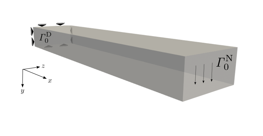
Cantilever, problem setup.
Study the setup shown in fig. 1 and the
comments in the input file solid_cantilever.py Run the simulation,
either in one of the provided Docker containers or using your own
FEniCSx/Ambit installation, using the command
mpiexec -n 1 python3 solid_cantilever.py
It is fully sufficient to use one core (mpiexec -n 1) for the
presented setup.
Open the results file results_solid_cantilever_displacement.xdmf in
Paraview, and visualize the deformation over time.
Figure 2 shows the displacement magnitude at the end of the simulation.
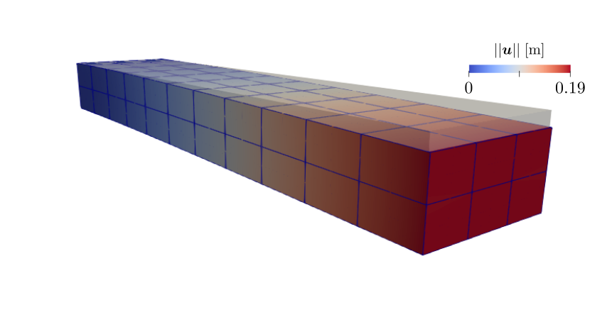
Cantilever, tip deformation. Color shows displacement magnitude.
Demo: Fluid
demos/fluid2D channel flow
This example shows how to set up 2D fluid flow in a channel around a rigid obstacle. Incompressible Navier-Stokes flow is solved using Taylor-Hood elements (9-node biquadratic quadrilaterals for the velocity, 4-node bilinear quadrilaterals for the pressure).

Channel flow, problem setup.
Study the setup and the comments in the input file fluid_channel.py.
Run the simulation, either in one of the provided Docker containers or
using your own FEniCSx/Ambit installation, using the command
mpiexec -n 1 python3 fluid_channel.py
It is fully sufficient to use one core (mpiexec -n 1) for the
presented setup.
results_fluid_channel_velocity.xdmf andresults_fluid_channel_pressure.xdmf in Paraview, and visualize the
velocity as well as the pressure over time.Fig. 4 shows the velocity magnitude (top) as well as the pressure (bottom part) at the end of the simulation.
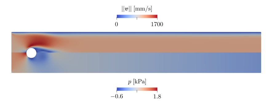
Velocity magnitude (top part) and pressure (bottom part) at end of simulation.
Demo: 0D flow
demos/flow0dSystemic and pulmonary circulation
This example demonstrates how to simulate a cardiac cycle using a
lumped-parameter (0D) model for the heart chambers and the entire
circulation. Multiple heart beats are run until a periodic state
criterion is met (which compares variable values at the beginning to
those at the end of a cycle, and stops if the relative change is less
than a specified value, here `eps_periodic' in the
TIME_PARAMS dictionary). The problem is set up such that periodicity
is reached after 5 heart cycles.
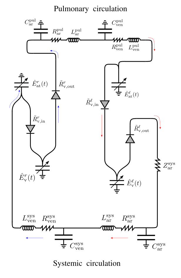
0D heart, systemic and pulmonary circulation, problem setup.
Study the setup in fig. 5 and the comments in
the input file flow0d_heart_cycle.py. Run the simulation, either in
one of the provided Docker containers or using your own FEniCSx/Ambit
installation, using the command
python3 flow0d_heart_cycle.py
For postprocessing of the time courses of pressures, volumes, and fluxes
of the 0D model, either use your own tools to plot the text output files
(first column is time, second is the respective quantity), or make sure
to have Gnuplot (and TeX) installed and navigate to the output folder
(tmp/) in order to execute the script flow0d_plot.py (which lies
in ambit/src/ambit_fe/postprocess/):
flow0d_plot.py -s flow0d_heart_cycle -n 100
plot_flow0d_heart_cycle is created inside tmp/. Look
at the results of pressures (\(p\)), volumes (\(V\)), and
fluxes (\(q\), \(Q\)) over time. Subscripts v, at,
ar, ven refer to ‘ventricular’, ‘atrial’, ‘arterial’, and
‘venous’, respectively. Superscripts l, r, sys, pul
refer to ‘left’, ‘right’, ‘systemic’, and ‘pulmonary’, respectively.
Try to understand the time courses of the respective pressures, as
well as the plots of ventricular pressure over volume. Check that the
overall system volume is constant and around 4-5 liters.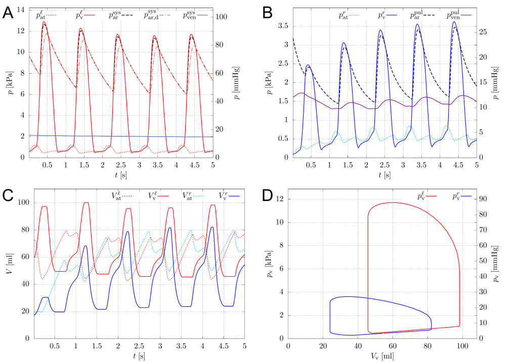
A. Left heart and systemic pressures over time. B. Right heart and pulmonary pressures over time. C. Left and right ventricular and atrial volumes over time. D. Left and right ventricular pressure-volume relationships of periodic (5th) cycle.
Demo: Solid + 0D flow
demos/solid_flow0d3D heart, coupled to systemic and pulmonary circulation
`order_disp' in the
FEM_PARAMS section from 1 to 2 (and increase
`quad_degree' to 6) such that quadratic finite element
ansatz functions (instead of linear ones) are used. While this will
increase accuracy and mitigate locking, computation time will
increase.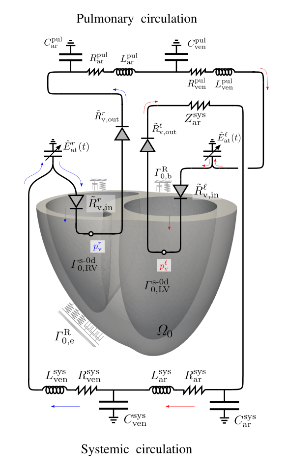
Generic 3D ventricular heart model coupled to a closed-loop systemic and pulmonary circulation model.
Study the setup shown in fig. 7 and the
comments in the input file solid_flow0d_heart_cycle.py. Run the
simulation, either in one of the provided Docker containers or using
your own FEniCSx/Ambit installation, using the command
mpiexec -n 1 python3 solid_flow0d_heart_cycle.py
It is fully sufficient to use one core (mpiexec -n 1) for the
presented setup, while you might want to use more (e.g.,
mpiexec -n 4) if you increase `order_disp' to 2.
Open the results file
results_solid_flow0d_heart_cycle_displacement.xdmf in Paraview, and
visualize the deformation over the heart cycle.
For postprocessing of the time courses of pressures, volumes, and fluxes
of the 0D model, either use your own tools to plot the text output files
(first column is time, second is the respective quantity), or make sure
to have Gnuplot (and TeX) installed and navigate to the output folder
(tmp/) in order to execute the script flow0d_plot.py (which lies
in ambit/src/ambit_fe/postprocess/):
flow0d_plot.py -s solid_flow0d_heart_cycle -V0 117e3 93e3 0 0 0
plot_solid_flow0d_heart_cycle is created inside tmp/.
Look at the results of pressures (\(p\)), volumes (\(V\)), and
fluxes (\(q\), \(Q\)) over time. Subscripts v, at,
ar, ven refer to ‘ventricular’, ‘atrial’, ‘arterial’, and
‘venous’, respectively. Superscripts l, r, sys, pul
refer to ‘left’, ‘right’, ‘systemic’, and ‘pulmonary’, respectively.
Try to understand the time courses of the respective pressures, as
well as the plots of ventricular pressure over volume. Check that the
overall system volume is constant and around 4-5 liters.number_of_cycles from 1 to 10 and re-run the
simulation. The simulation will stop when the cycle error (relative
change in 0D variable quantities from beginning to end of a cycle)
falls below the value of `eps_periodic' (set to
\(5 \%\)). How many cycles are needed to reach periodicity?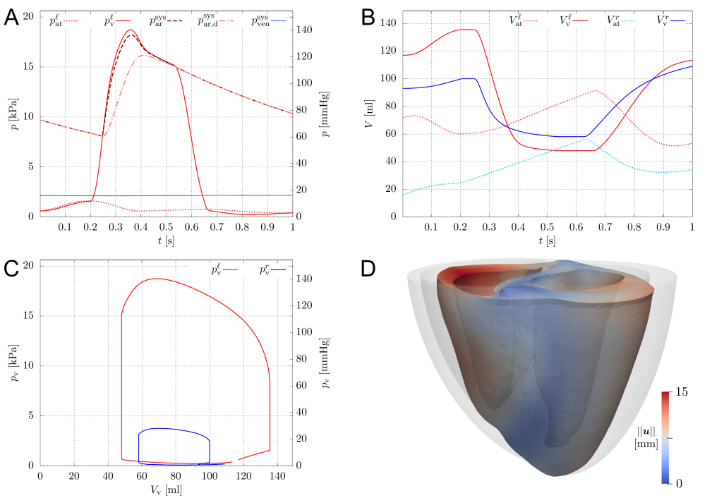
A. Left heart and systemic pressures over time. B. Left and right ventricular and atrial volumes over time. C. Left and right ventricular pressure-volume relationships. D. Snapshot of heart deformation at end-systole, color indicates displacement magnitude.
Demo: Fluid + 0D flow
demos/fluid_flow0dBlocked pipe flow with 0D model bypass

Blocked pipe with 0D model bypass, simulation setup.
Study the setup shown in fig. 9 and the
comments in the input file fluid_flow0d_pipe.py. Run the simulation,
either in one of the provided Docker containers or using your own
FEniCSx/Ambit installation, using the command
mpiexec -n 1 python3 fluid_flow0d_pipe.py
It is fully sufficient to use one core (mpiexec -n 1) for the
presented setup.
Open the results file results_fluid_flow0d_pipe_velocity.xdmf in
Paraview, and visualize the velocity over time.

Streamlines of velocity at end of simulation, color indicates velcity magnitude.
Demo: FSI
demos/fsiChannel flow around elastic flag
\[\begin{aligned} \boldsymbol{v}_{\text{f}}= \bar{v}(t,y) \boldsymbol{e}_{x} \quad & \text{on}\; \mathit{\Gamma}_{t,\mathrm{in}}^{D,\text{f}} \times [0,T], \label{eq:flag_dbc_in} \end{aligned}\]with
\[\begin{split}\begin{aligned} \bar{v}(t,y) = \begin{cases} 1.5 \,\bar{U}\, \frac{y(H-y)}{\left(\frac{H}{2}\right)^2} \frac{1-\cos\left(\frac{\pi}{2}t\right)}{2}, & \text{if} \; t < 2, \\ 1.5 \,\bar{U}\, \frac{y(H-y)}{\left(\frac{H}{2}\right)^2}, & \text{else}, \end{cases} \label{eq:flag_dbcs_func} \end{aligned}\end{split}\]
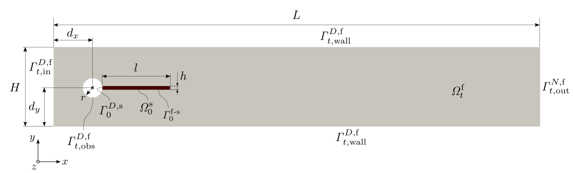
Geometrical parameters, given in \([\mathrm{mm}]\), are:
\(L\) |
\(H\) |
\(r\) |
\(l\) |
\(h\) |
\(d_x\) |
\(d_y\) |
|---|---|---|---|---|---|---|
2500 |
410 |
50 |
350 |
20 |
200 |
200 |
fsi_channel_flag.py. Run the simulation for FSI2 and
FSI3 cases, either in one of the provided Docker containers or using
your own FEniCSx/Ambit installation, using the commandmpiexec -n 1 python3 fsi_channel_flag.py
mpiexec -n 4)
in order to speed up the simulation a bit.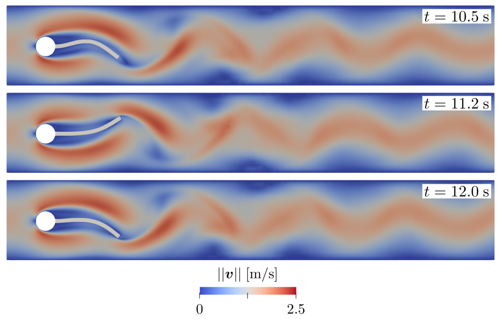
FSI2 case: Magnitude of fluid velocity at three instances in time (\(t=10.5\;\mathrm{s}\), \(t=11.2\;\mathrm{s}\), and \(t=12\;\mathrm{s}\)) towards end of simulation, color indicates velcity magnitude.
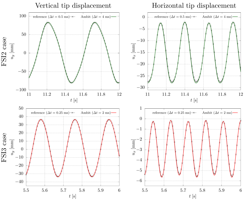
Comparison to benchmark reference solution for the time course of the flag’s tip displacement for the two setups FSI2 and FSI3. A fairly coarse time step of \(\Delta t = 4 \;\mathrm{ms}\) (FSI2) and \(\Delta t = 2 \;\mathrm{ms}\) (FSI3) already allows a close match to the original results.
Demo: Multiphase fluid
demos/fluid_multiphaseRising bubble under gravity
We study a 2D multiphase flow benchmark, where two incompressible fluids of different densities and different viscosities interact: a fluid of lower density (and viscosity) is immersed into a surrounding fluid of higher density (and viscosity), and a gravitational force acts in vertical direction, cf. the setup in Fig. 14. This setup corresponds to the benchmark case described in [BtE26],:cite:p:ten-eikelder2024. The following Dirichlet boundary conditions apply:
The body force term takes the form \(\hat{\boldsymbol{b}}=-\rho\boldsymbol{g}\), with \(\boldsymbol{g}\cdot\boldsymbol{e}_{y}=0.98\). Our phase field variable is bounded between \(a=-1\) and \(b=1\). Further, Cahn-Hilliard parameters are chosen as
with \(\tilde{\sigma}=\frac{3\sigma}{2\sqrt{2}}\) (surface energy density coefficient) and \(\epsilon=0.64\,h_{\mathrm{e}}\), where \(h_{\mathrm{e}}\) is the finite element edge length. The mobility exponent in Eq. ([equation-mobility]) is chosen to \(\gamma=1\). Parameters for the two cases are shown in the following table. Bulk viscosities are assumed zero (\(\zeta=0\)).
rho_1 |
rho_2 |
eta_1 |
eta_2 |
sigma |
|
|---|---|---|---|---|---|
Case 1 |
1000 |
100 |
10 |
1 |
24.5 |
Case 2 |
1000 |
1 |
10 |
0.1 |
1.96 |
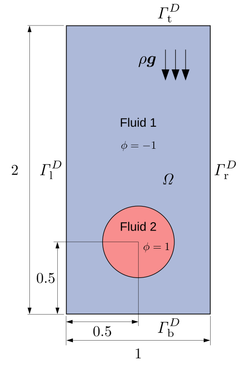
Rising bubble benchmark [BtE26],:cite:p:ten-eikelder2024: A fluid with lower density (fluid 2) is surrounded by a fluid of higher density (fluid 1). Bottom and top velocities are constrained, as well as the normal velocity on the left and right walls. A gravitational force acts in vertical direction.
Study the setup shown in Fig. 14 together
with the parameters in the table and the comments in the input file
fluid_multiphase_rising_bubble.py. Run the simulation for both cases
1 and 2, either in one of the provided Docker containers or using your
own FEniCSx/Ambit installation, using the command
mpiexec -n 1 python3 fluid_multiphase_rising_bubble.py
meshsize inside
mesh_domain (increase from [32,64] to [64,128] to
[128,256]; the first value is the number of elements used in
horizontal, the second the number in vertical direction). If your
system allows, use more than one core, especially for finer mesh sizes
(hence run with mpiexec -n 4 ... or more). A good rule of thumb is
to have 10000–20000 degrees of freedom per process. The time step and
the interface thickness parameter \(\epsilon\) will be changed
automatically depending on the chosen mesh size. Compare the results
for the two cases and the different mesh sizes.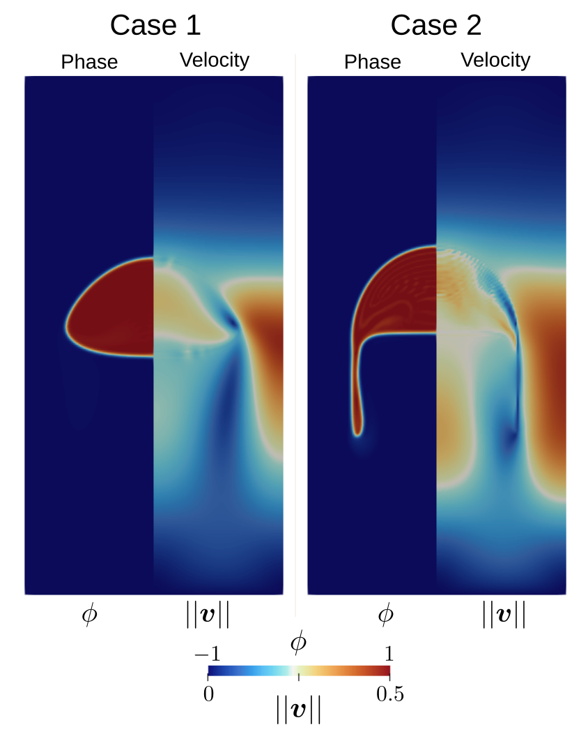
Phase field \(\phi\) (left part) and magnitude of velocity \(||\boldsymbol{v}||\) (right part) solutions for both cases at the final time \(t=3.0\).
Figure 16 plots the center of mass as well as the rise velocity of the lower-density fluid bubble over time (mesh size \(128 \times 256\)) and compares the solution with two different reference solutions (one a mass-, the other a volume-averaged velocity formulation) from Brunk and ten Eikelder [BtE26] as well as ten Eikelder and Schillinger [tES24]. We observe good agreements between our (mass-averaged velocity) solution and the volume-averaged velocity reference solutions. Slight deviations to the mass-averaged reference solutions are observed.
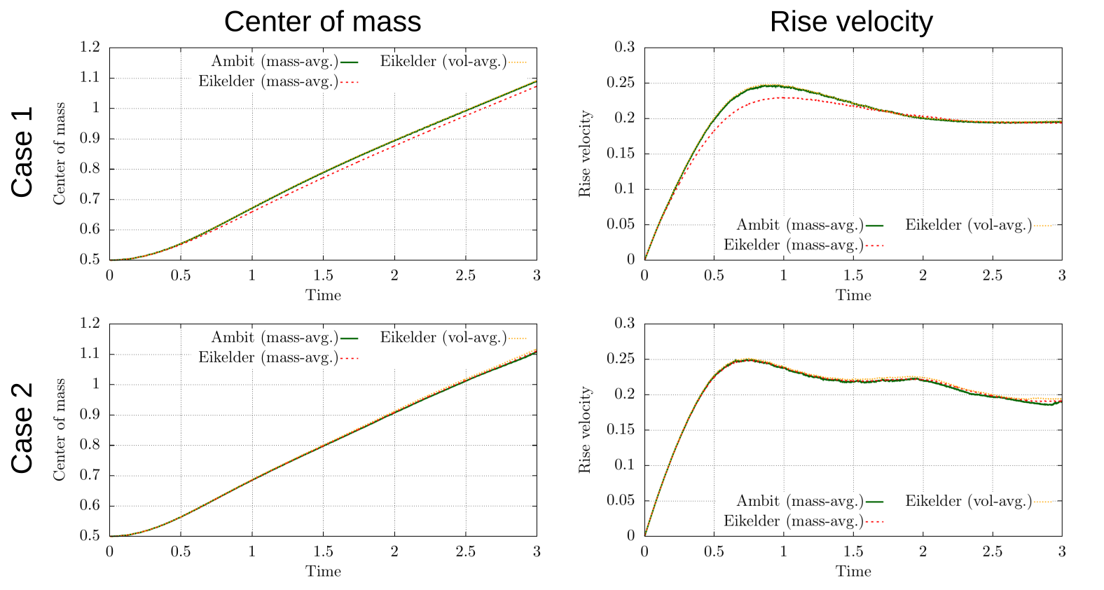
Center of mass (left column) and rise velocity (right column) for both cases over time, comparison to reference solutions from Brunk and ten Eikelder [BtE26].
Table of symbols
C. J. Arthurs, K. D. Lau, K. N. Asrress, S. R. Redwood, and C. A. Figueroa. A mathematical model of coronary blood flow control: simulation of patient-specific three-dimensional hemodynamics during exercise. Am J Physiol Heart Circ Physiol, 310(9):H1242–H1258, 2016. doi:10.1152/ajpheart.00517.2015.
S. Balay, S. Abhyankar, M. F. Adams, S. Benson, J. Brown, P. Brune, K. Buschelman, E. Constantinescu, L. Dalcin, A. Dener, V. Eijkhout, W. D. Gropp, V. Hapla, T. Isaac, P. Jolivet, D. Karpeev, D. Kaushik, M. G. Knepley, F. Kong, S. Kruger, D. A. May, L. C. McInnes, R. T. Mills, L. Mitchell, T. Munson, J. E. Roman, K. Rupp, P. Sanan, J. Sarich, B. F. Smith, S. Zampini, H. Zhang, H. Zhang, and J. Zhang. PETSc/TAO users manual. Technical Report ANL-21/39 - Revision 3.17, Argonne National Laboratory, 2022.
A. Brunk and M. F. P. ten Eikelder. A simple, fully-discrete, unconditionally energy-stable method for the two-phase Navier-Stokes Cahn-Hilliard model with arbitrary density ratios. Journal of Computational Physics, 548():114558, 2026. doi:10.1016/j.jcp.2025.114558.
D. Chapelle, P. Le Tallec, P. Moireau, and M. Sorine. Energy-preserving muscle tissue model: formulation and compatible discretizations. Journal for Multiscale Computational Engineering, 10(2):189–211, 2012. doi:10.1615/IntJMultCompEng.2011002360.
C. Farhat, P. Avery, T. Chapman, and J. Cortial. Dimensional reduction of nonlinear finite element dynamic models with finite rotations and energy-based mesh sampling and weighting for computational efficiency. International Journal for Numerical Methods in Engineering, 98(9):625–662, 2014. doi:10.1002/nme.4668.
M. W. Gee, Ch. Förster, and W. A. Wall. A computational strategy for prestressing patient-specific biomechanical problems under finite deformation. International Journal for Numerical Methods in Biomedical Engineering, 26(1):52–72, 2010. doi:10.1002/cnm.1236.
M. W. Gee, C. T. Kelley, and R. B. Lehoucq. Pseudo-transient continuation for nonlinear transient elasticity. International Journal for Numerical Methods in Engineering, 78(10):1209–1219, 2009. doi:10.1002/nme.2527.
J. M. Guccione, K. D. Costa, and A. D. McCulloch. Finite element stress analysis of left ventricular mechanics in the beating dog heart. J Biomech, 28(10):1167–1177, 1995. doi:10.1016/0021-9290(94)00174-3.
S. Göktepe, O. J. Abilez, K. K. Parker, and E. Kuhl. A multiscale model for eccentric and concentric cardiac growth through sarcomerogenesis. J Theor Biol, 265(3):433–442, 2010. doi:10.1016/j.jtbi.2010.04.023.
M. Hirschvogel. Computational modeling of patient-specific cardiac mechanics with model reduction-based parameter estimation and applications to novel heart assist technologies. Verlag Dr. Hut, MediaTUM, 1 edition, 2019. URL: https://mediatum.ub.tum.de/1445317.
M. Hirschvogel, M. Balmus, M. Bonini, and D. Nordsletten. Fluid-reduced-solid interaction (FrSI): physics- and projection-based model reduction for cardiovascular applications. Journal of Computational Physics, 506:112921, 2024. URL: https://www.sciencedirect.com/science/article/pii/S0021999124001700, doi:10.1016/j.jcp.2024.112921.
M. Hirschvogel, M. Bassilious, L. Jagschies, S. M. Wildhirt, and M. W. Gee. A monolithic 3D-0D coupled closed-loop model of the heart and the vascular system: Experiment-based parameter estimation for patient-specific cardiac mechanics. Int J Numer Method Biomed Eng, 33(8):e2842, 2017. doi:10.1002/cnm.2842.
Marc Hirschvogel. Ambit – A FEniCS-based cardiovascular multi-physics solver. Journal of Open Source Software, 9(93):5744, 2024. URL: https://doi.org/10.21105/joss.05744, doi:10.21105/joss.05744.
G. A. Holzapfel. Nonlinear Solid Mechanics – A Continuum Approach for Engineering. Wiley Press Chichester, 2000.
G. A. Holzapfel and R. W. Ogden. Constitutive modelling of passive myocardium: A structurally based framework for material characterization. Phil Trans R Soc A, 367(1902):3445–3475, 2009. doi:10.1098/rsta.2009.0091.
A. Logg, K.-A. Mardal, and G. N. Wells, editors. Automated Solution of Differential Equations by the Finite Element Method – The FEniCS Book. Springer, 2012. ISBN 978-3-642-23098-1. doi:10.1007/978-3-642-23099-8.
D. A. Nordsletten, M. McCormick, P. J. Kilner, P. Hunter, D. Kay, and N. P. Smith. Fluid-solid coupling for the investigation of diastolic and systolic human left ventricular function. International Journal for Numerical Methods in Biomedical Engineering, 27(7):1017–1039, 2011. doi:10.1002/cnm.1405.
A. Schein and M. W. Gee. Greedy maximin distance sampling based model order reduction of prestressed and parametrized abdominal aortic aneurysms. Advanced Modeling and Simulation in Engineering Sciences, 8(18):, 2021. doi:10.1186/s40323-021-00203-7.
M. F. P. ten Eikelder and D. Schillinger. The divergence-free velocity formulation of the consistent Navier-Stokes Cahn-Hilliard model with non-matching densities, divergence-conforming discretization, and benchmarks. Journal of Computational Physics, 513():113148, 2024. doi:10.1016/j.jcp.2024.113148.
T. E. Tezduyar and Y. Osawa. Finite element stabilization parameters computed from element matrices and vectors. Computer Methods in Applied Mechanics and Engineering, 190(3–4):411–430, 2000. doi:10.1016/S0045-7825(00)00211-5.
S. Turek and J. Hron. Proposal for numerical benchmarking of fluid-structure interaction between an elastic object and laminar incompressible flow. In H.-J.Bungartz and M. Schäfer, editors, Lecture Notes in Computational Science and Engineering, volume 53, pages 371–385. Springer Berlin Heidelberg, 2006. doi:10.1007/3-540-34596-5\_15.
N. Westerhof, J.-W. Lankhaar, and B. E. Westerhof. The arterial Windkessel. Med Biol Eng Comput, 47(2):H81–H88, 2009. doi:10.1007/s11517-008-0359-2.